Goals and Motivation

Vector data are one of the fundamental GIS data types and one of the first incorporated into R. R has several packages for working with vector data and we will cover these packages in this section. But first we will provide a short review of vector data.

By the end of this lesson, you should be able to:

• Understand and describe the main features and types of vector data.
• Generate point data from a set of latitudes and longitudes (e.g., fields sites).
• Read, write, query, and manipulate vector data using the sp package.
• Read, write, query, and manipulate vector data using the sf package.

Points, lines, and polygons!

These data are a way of representing real-world features on a landscape in a highly simplified way. The simplest of these features is a point, which is a 0-dimensional feature that can be used to represent a specific location on the earth, such as a single tree or an entire city. Linear, 1-dimensional features can be represented with points (or vertices) that are connected by a path to form a line and when many points are connected these form a polyline. Finally, when a polyline’s path returns to its origin to represent an enclosed space, such as a forest, watershed boundary, or lake, this forms a polygon.

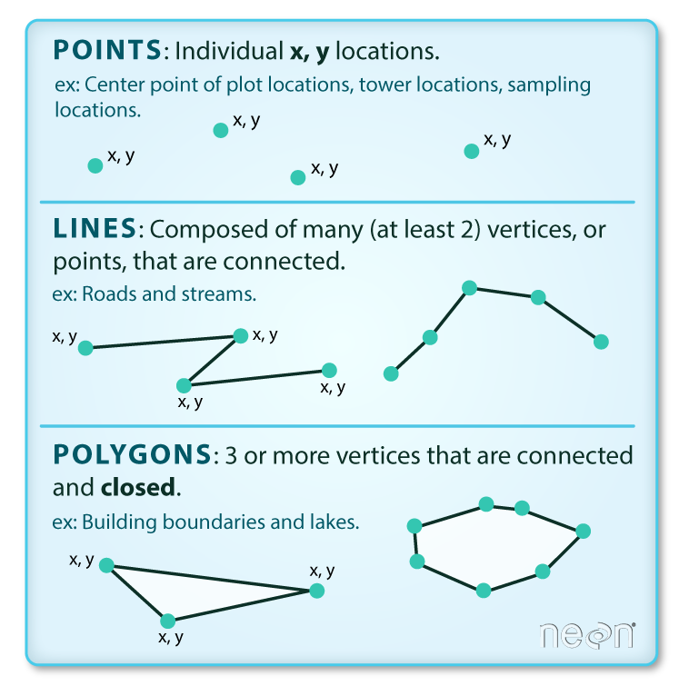
Image from: https://earthdatascience.org/courses/earth-analytics/spatial-data-r/intro-vector-data-r/

Excercise

We will explore vector data objects in R by first starting a new R Markdown.

• In the project you created for this workshop, open a fresh R Markdown file (File > New File > R Markdown).
• Name it ‘Vector data’ and save it in your project.

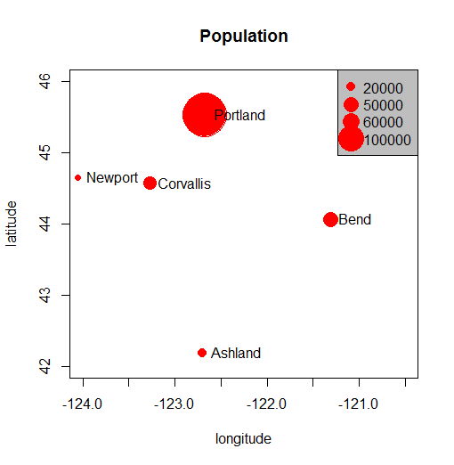
We can represent these features in R without actually using GIS packages. In this example, we’ll represent several cities in Oregon with common R data structures that you are probably already familiar with.

cities <- c('Ashland','Corvallis','Bend','Portland','Newport')
longitude <- c(-122.699, -123.275, -121.313, -122.670, -124.054)
latitude <- c(42.189, 44.57, 44.061, 45.523, 44.652)
population <- c(20062,50297,61362,537557,9603)
locs <- cbind(longitude, latitude) 
plot(locs, cex=sqrt(population*.0002), pch=20, col='red', 
  main='Population', xlim = c(-124,-120.5), ylim = c(42, 46))
text(locs, cities, pos=4)

Add a legend…

breaks <- c(20000, 50000, 60000, 100000)
options(scipen=3)
legend("topright", legend=breaks, pch=20, pt.cex=1+breaks/20000, 
  col='red', bg='gray')

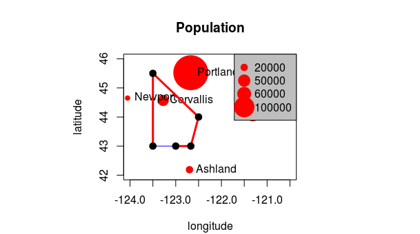
Add some more points, some lines, and a polygon to our map…

lon <- c(-123.5, -123.5, -122.5, -122.670, -123)
lat <- c(43, 45.5, 44, 43, 43)
x <- cbind(lon, lat)
polygon(x, border='blue')
lines(x, lwd=3, col='red')
points(x, cex=2, pch=20)

So, is this sufficient for working with spatial data in R and doing spatial analysis? What are we missing? If you have worked with vector data before, you may know that these data also usually have:

• A coordinate reference system
• A bounding box or extent
• Plot order
• Data

In the next section we will introduce the sp package that will allow us to take fuller advantage of spatial features in R.