Goals and Motivation

Rasters are the other fundamental GIS data format and one that works very will in R. the prefered method far and away is to use the raster package by Robert J. Hijmans. The raster package has made working with raster data (as well as vector spatial data for some things) much easier and more efficient. The raster package allows you to:

• read and write almost any commonly used raster data format using rgdal
• create rasters, do typical raster processing operations such as resampling, projecting, filtering, raster math, etc.
• work with files on disk that are too big to read into memory in R
• run operations quite quickly since the package relies on back-end C code

The home page for the raster package has links to several well-written vignettes and documentation for the package.

The raster package uses three classes / types of objects to represent raster data - RasterLayer, RasterStack, and RasterBrick - these are all S4 new style classes in R, just like sp classes.

All that said, raster has not been updated in the last year - there has been discussion in the R spatial developer world among several folks of updating / modifying raster to be both sf and pipe-based workflow friendly - it looks like this is coalescing in the stars: spatiotemporal tidy arrays for R package being developed by Edzer Pebezma, Michael Sumer, and Etienne Racine. Their proposal outlines the approach they are taking - you can play with the development version but it is still very much in alpha stages.

By the end of this module, you will:

• Understand how to create, load, and analyze raster data in R
• Understand basic structure of rasters in R and how to manipulate
• Be able to conduct operations on raster data, such as zonal statistics

We will explore raster objects in R by first starting a new R Markdown.

In the project you created for this workshop, open a fresh R Markdown file (File > New File > R Markdown). Name it ‘raster data’ and save it in your project.

Rasters

Let’s create an empty RasterLayer object - we have to define the matrix (rows and columns) the spatial bounding box, and then we provide values to the cells using the runif function to derive random values from the uniform distribution.

library(raster)
r <- raster(ncol=10, nrow = 10, xmx=-116,xmn=-126,ymn=42,ymx=46)
str(r)
r
r[] <- runif(n=ncell(r))
r
plot(r)

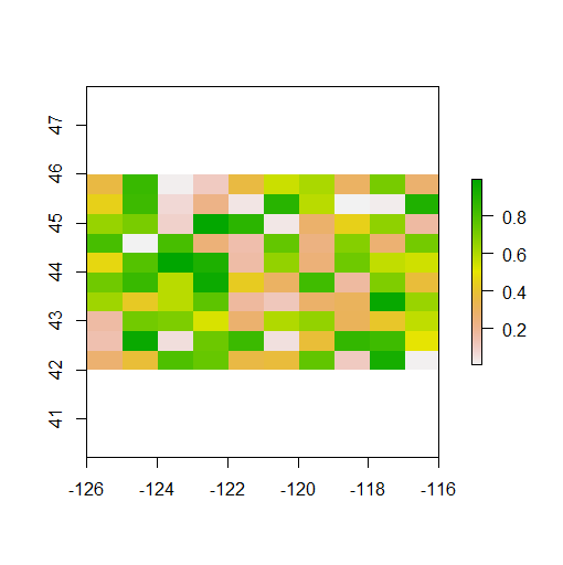
When you look at summary information for the RasterLayer, by simply typing “r”, you’ll notice the main information defining a RasterLayer object described. Minimal information needed to define a RasterLayer include the number of columns and rows, the bounding box or spatial extent of the raster, and the coordinate reference system. What do you notice about the coordinate reference system of the raster we just generated from scratch?

An important feature of the raster package is that when you load a raster, it is not actually loaded into memory. However, this raster we made from scratch is in memory but very small. Instead, it reads information about the raster into memory, such as its dimensions, its extent, and more. This makes loading and working with rasters as it will only ever load into memory what is needed for a specific task. For example, you can access raster values via direct indexing or line/column indexing. The raster package accesses just those locations on the disk. Take a minute to see how this works using raster r we just created - the syntax is:

r[i]
r[line, column]

RasterStacks

A RasterStack is a raster object with multiple raster layers - essentially a multi-band raster. RasterStack and RasterBrick are very similar and we won’t delve into differences much here - basically, a RasterStack can virtually connect several RasterLayer objects in memory and allows pixel-based calculations on separate raster layers, while a RasterBrick has to refer to a single multi-layer file or multi-layer object. Note that methods that operate on either a RasterStack or RasterBrick usually return a RasterBrick, and processing will be mor efficient on a RasterBrick object.

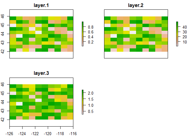
It’s easy to manipulate our RasterLayer to make a couple new layers, and then stack layers:

r2 <- r * 50
r3 <- sqrt(r * 5)
s <- stack(r, r2, r3)
s
plot(s)

Same process for generating a raster brick (here I make layers and create a RasterBrick in same step):

b <- brick(x=c(r, r * 50, sqrt(r * 5)))
b

In the next section, we’ll work with real raster data and do exploratory analyses.