Extracting Data from Rasters
In this section, we’ll learn how to pull useful information from raster datasets. These will include generic functions to summarize rasters as a whole or to extract information based on the boundaries of a second layer.
Lesson Goals
By the end of this section you will be able to:
- Extract summary stats for a raster or stack of rasters
- Extract raster values at sample points
- Delineate a watershed and extract a summary of raster values within the boundary
- Bonus Excercise - Delineate several watersheds and extract raster metrics within watershed boundaries
Excercise 1: Raster and RasterBrick summary stats
We can also extract potentially useful information from a raster layer using several methods.
library(raster)
#Reading
cal_elev <- raster('./data/cal_elev.tif')
cellStats(cal_elev, stat='mean')
quantile(cal_elev, probs = c(0.25, 0.5, 0.75))
#[1] 300.048
#    25%       50%       75%
#85.35121 161.22613 408.62559
Many of these methods work with RasterBricks as well (although some of these stats may not be relevant for some of the layers, such as flowdir).
cellStats(cal_terrain, stat='mean')
quantile(cal_terrain, probs = c(0.25, 0.5, 0.75))
#        tri         tpi   roughness       slope      aspect     flowdir
# 9.64157210 -0.09001769 31.13302748  0.12417778  3.29963730 34.03649593
#                   25%         50%        75%
#tri        0.793477233  5.29052019 15.7185688
#tpi       -1.321671745 -0.10031628  0.9763394
#roughness  2.317155757 17.19726370 50.9859111
#slope      0.007261573  0.06209942  0.2085050
#aspect     1.442969122  3.60642750  5.0135436
#flowdir    4.000000000 16.00000000 64.0000000
Excercise 2: Extracting raster data at points
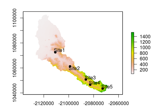
Let’s pretend we have 5 sample sites within the Calapooia River basin and we’d like to know the elevation of those sites. In this scenario, we only have the latitude and longitude of each site.
#Read in sample  sites table
sites <- read.csv('./data/calapooia-samples.csv')
#A different flavor of importing coordinates to a spatial object
coordinates(sites) <- c('Lon','Lat')
proj4string(sites) <- "+proj=longlat +datum=WGS84
                       +no_defs +ellps=WGS84 +towgs84=0,0,0"
#CRS of points and raster must match
sites <- spTransform(sites, CRS(proj4string(cal_elev)))
#Plot to verify
plot(cal_elev)
plot(sites, add = T, pch = 19)
library(maptools)
pointLabel(coordinates(sites),labels=sites$SampleID)
We can use extract to get elevations at out sample sites. This function returns a vector, so we can simply add the results on as a new column in sites.
sites$elevation <- extract(cal_elev, sites)
sites@data
#  SampleID elevation
#1    Site1  133.6236
#2    Site2  192.2931
#3    Site3  423.4795
#4    Site4  489.0032
#5    Site5  679.1790
Excercise 3: Extracting data by polygon
Creating summaries within a polygon is a common and important analysis in GIS, especially in water resources where watershed summaries are often used to understand why freshwater environments differ from one another. Let’s say you want to get the watershed for site 1 and calculate watershed metrics for it. The USGS has an online tool that can delineate the watershed for this point called StreamStats. It is worth exploring the point-and-click version. The StreamStat Service API is exposed, meaning we can build simple text URLs that can be submitted to the server as a query. We won’t go into detail for this excercise. First, we need to import the custom function
library(jsonlite);library(sf);library(sp);library(geojsonio)
#Define function - watershed
watershed = function(state, lon, lat){
  p1 = 'https://streamstats.usgs.gov/streamstatsservices/watershed.geojson?rcode='
  p2 = '&xlocation='
  p3 = '&ylocation='
  p4 = '&crs=4326&includeparameters=false&includeflowtypes=false&includefeatures=true&simplify=true'
  query <-  paste0(p1, state, p2, toString(lon), p3, toString(lat), p4)
  mydata <- fromJSON(query, simplifyVector = FALSE, simplifyDataFrame = FALSE)
  poly_geojsonsting <- toJSON(mydata$featurecollection[[2]]$feature, auto_unbox = TRUE)
  poly <- geojson_sp(poly_geojsonsting)
  poly
}
Now that the function is defined, we can provide it with the information about our site to delineate its watershed.
state <- 'OR'
latitude <- 44.39460
longitude <- -122.9248
# Delineate the watershed
ws <- watershed('OR', longitude, latitude)
# Plot on top of Calapooia basin for context
cal_ws <- readOGR(dsn = './data', layer = 'calapooia-ws')
plot(cal_ws)
plot(ws, add = T, border='red')
Let’s generate watershed summaries for the terrain stack we generated before. First, we’ll need to read it in and then make sure that the watershed boundary and our raster data are in the same CRS. Finally, we’ll generate summary stats for the watershed.
cal_terrain <-  readRDS('./data/cal_terrain.rds')
proj4string(ws) == proj4string(cal_terrain)
#Project to match cal_terrain
ws <- spTransform(ws, CRS(proj4string(cal_terrain)))
metrics <- extract(cal_terrain, ws, fun = 'mean', na.rm = T, small = T)
print(metrics)
#          tri        tpi roughness     slope   aspect flowdir
#[1,] 13.66916 -0.1562615  44.41507 0.1829341 3.616169 16.9229
Bonus Excercise - Multi-watershed delineation and metric calculation
We may not have time to cover this section. However, we thought it would be useful to at least provide the code to delineate multiple watersheds at once and calculate summary metrics. Doing so requires a for loop in which we select out each point at a time, submit its coordinates to the online service, and extract the summary metrics for the returned watershed boundary.
#Read in the points table
pts <- read.csv('./data/calapooia-samples.csv')
#Loop through each point where each point is a in the table
for(i in 1:nrow(pts)){
  print(i)
  pt <- pts[i, ] #select row i from table
  #Use info from that row to delin watershed
  wstmp <- watershed(pt$State, pt$Lon, pt$Lat)
  #Make sure they're in the same CRS
  wstmp <- spTransform(wstmp, CRS(proj4string(cal_terrain)))
  #Add a sample ID column to new watershed
  wstmp$SampleID <- pt$SampleID
  #Remove all unnecessary columns
  wstmp <- wstmp[, 'SampleID']
  #Use extract on raster brick
  metrics <- extract(cal_terrain, wstmp, fun = 'mean', na.rm = T, small = T)
  #Use cbind to attach new data to the watershed attribute table
  wstmp@data <- cbind(wstmp@data, metrics)
  #If it's the first time in loop, create the final output
  if(i == 1){
    cal_ws <- wstmp
  }else{
    #Otherwise, append the new watershed to previous watershed
    cal_ws <- rbind(cal_ws, wstmp)
  }
}
#Plot to see if it worked
plot(cal_elev)
plot(cal_ws, add = T)
plot(sites, add = T, pch=20)
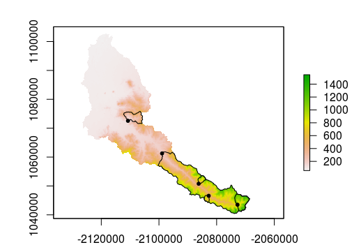
In addition to delineating the watersheds, the loop used the extract function with fun = mean to calculate the mean of each of the layers in the RasterBrick cal_terrain:
cal_ws@data
#  SampleID      tri        tpi roughness     slope   aspect  flowdir
#1    Site1 13.66916 -0.1562616  44.41507 0.1829341 3.616169 16.92290
#2    Site2 23.77488 -0.2711316  76.93438 0.3058251 3.055297 35.13301
#3    Site3 33.14047 -0.4726615 109.41227 0.4170104 3.682443 10.22483
#4    Site4 32.54499 -1.2240693 103.42906 0.4042515 2.562071 41.04296
#5    Site5 26.20215 -0.5688954  84.08578 0.3346428 3.625224 21.49765